Gradient Descent: How It Works, Types, and Practical Implementation

What Is Gradient Descent?

Gradient descent is an iterative optimization algorithm used to minimize a function by repeatedly adjusting its parameters in the direction of steepest decrease. In machine learning, it serves as the primary method for training models by finding the set of parameters that produce the lowest possible error on training data.

The algorithm computes the gradient of a loss function with respect to each parameter, then updates those parameters proportionally in the opposite direction of the gradient.

The core intuition is straightforward. Imagine standing on a mountainside in dense fog, unable to see the valley below. The best strategy for reaching the lowest point is to feel the slope under your feet and take a step downhill. Gradient descent does exactly this, but in a mathematical space that may have millions of dimensions. At each step, the algorithm evaluates the slope of the loss surface at the current position and moves the parameters toward lower loss values.

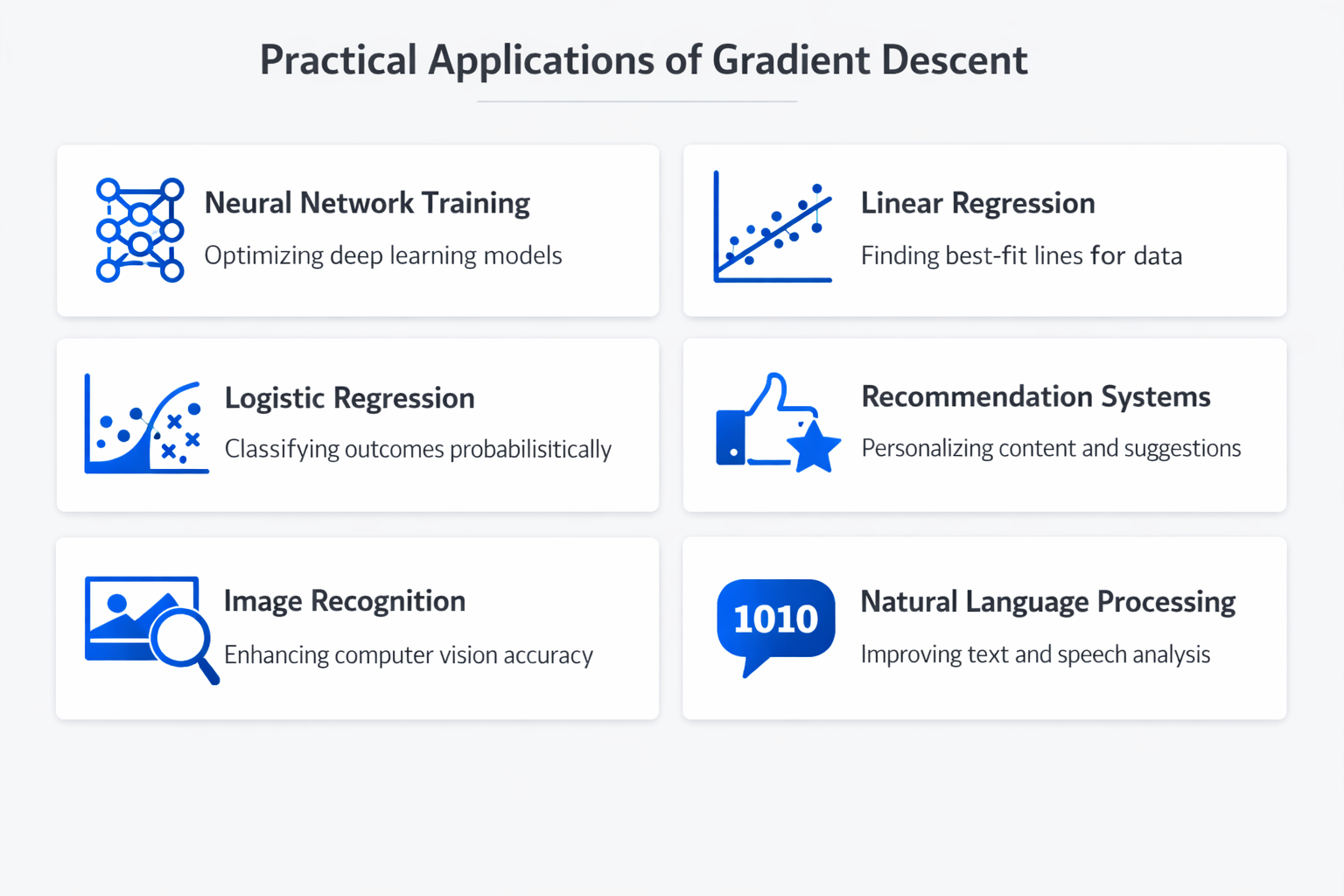
Gradient descent is foundational to virtually every area of modern artificial intelligence. It powers the training of neural networks, linear regression models, logistic classifiers, and many other architectures.

Without an efficient optimization method like gradient descent, the parameters of complex models could not be learned from data, and the entire field of deep learning would not exist in its current form.

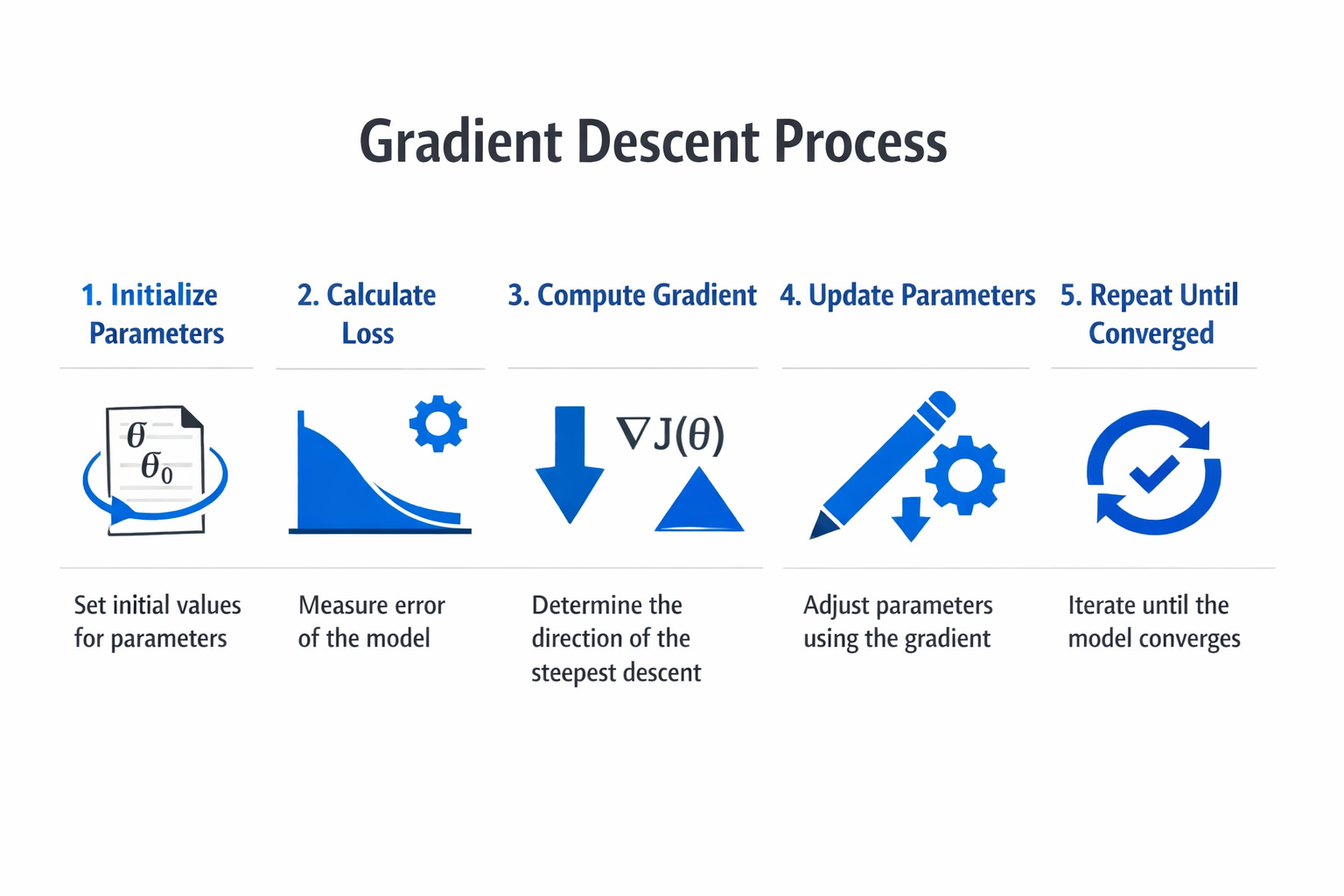
How Gradient Descent Works

The mechanics of gradient descent involve a repeating cycle of evaluation, computation, and adjustment. Each cycle brings the model parameters closer to values that minimize the loss function.

Defining the Loss Function

Every gradient descent process begins with a loss function, also called a cost function or objective function. The loss function measures how far the model's predictions are from the actual target values. For regression tasks, mean squared error is a common choice. For classification tasks, cross-entropy loss is standard.

The loss function takes the model's current parameters as input and returns a single scalar value representing the total error. The goal of gradient descent is to find the parameter values that make this scalar as small as possible.

Computing the Gradient

The gradient is a vector of partial derivatives, one for each parameter in the model. Each partial derivative measures how much the loss would change if that specific parameter were nudged by a tiny amount. A large partial derivative means the loss is highly sensitive to changes in that parameter. A small one means the parameter has little effect on the current loss.

For simple models like linear regression, the gradient can be computed analytically using calculus.

For complex models like convolutional neural networks or transformer models, the gradient is computed using the backpropagation algorithm, which applies the chain rule of calculus efficiently across all layers of the network.

The Update Rule

Once the gradient is known, the parameters are updated using a simple rule: subtract the gradient multiplied by a scalar called the learning rate. In mathematical notation, the update for each parameter w is:

w = w - learning_rate * gradient

The learning rate controls the size of each step. A large learning rate takes big steps, which can speed up convergence but risks overshooting the minimum and causing the loss to diverge. A small learning rate takes cautious steps, which provides stability but may result in extremely slow convergence or getting trapped in suboptimal regions of the loss surface.

Iterating Until Convergence

The gradient computation and parameter update repeat for many iterations. Each iteration is called a training step. A full pass through the entire training dataset is called an epoch, and training typically runs for many epochs. With each step, the loss should decrease, indicating the model is improving its predictions.

Training stops when a convergence criterion is met. Common criteria include the loss falling below a threshold, the loss change between iterations becoming negligibly small, or a fixed number of epochs being reached. In practice, data splitting into training and validation sets allows practitioners to monitor whether the model generalizes well to unseen data, not just the data it was trained on.

Types of Gradient Descent

Gradient descent comes in three primary variants, each defined by how much data is used to compute the gradient at each step. The choice among them involves tradeoffs between computational cost, convergence speed, and optimization stability.

Batch Gradient Descent

Batch gradient descent computes the gradient using the entire training dataset at every step. This produces the most accurate estimate of the true gradient, resulting in smooth and stable convergence toward the minimum. For convex loss functions, batch gradient descent is guaranteed to converge to the global minimum given a sufficiently small learning rate.

The primary drawback is computational cost. When the training dataset contains millions of examples, computing the full gradient at every step becomes prohibitively expensive. Batch gradient descent also requires the entire dataset to fit in memory, which limits its applicability to large-scale problems. For small to medium datasets, however, it remains a reliable and predictable choice.

Stochastic Gradient Descent (SGD)

Stochastic gradient descent computes the gradient using a single randomly selected training example at each step. This makes each update extremely fast and allows the algorithm to begin improving the model before processing the full dataset. SGD also introduces noise into the gradient estimates, which can help the optimizer escape shallow local minima and saddle points.

The tradeoff is that individual updates are noisy and the loss can fluctuate significantly from step to step. The optimization path is erratic compared to batch gradient descent. Despite this, SGD often reaches good solutions faster in wall-clock time, especially on large datasets. The noise can also serve as implicit regularization, improving the model's ability to generalize.

SGD is the historical foundation of training algorithms in supervised learning and remains widely used today.

Mini-Batch Gradient Descent

Mini-batch gradient descent splits the difference between batch and stochastic methods by computing the gradient on a small random subset of the training data, called a mini-batch. Typical mini-batch sizes range from 32 to 512 examples. This approach is the default in modern deep learning practice.

Mini-batch gradient descent offers several advantages. It reduces the variance of gradient estimates compared to SGD while remaining far more computationally efficient than full-batch gradient descent. It also leverages vectorized computation on GPUs, which are optimized for parallel operations on batches of data. The mini-batch size is a hyperparameter that affects both training speed and model performance.

Larger batches provide more stable gradients but may converge to sharper minima that generalize less well.

Advanced Optimizers Built on Gradient Descent

The basic gradient descent update rule has been extended by a family of adaptive optimization algorithms. These methods modify how gradients are used to update parameters, often achieving faster and more reliable convergence.

- SGD with Momentum accumulates a moving average of past gradients, allowing the optimizer to build velocity in consistent gradient directions and dampen oscillations.

- AdaGrad adapts the learning rate for each parameter individually, using larger updates for infrequent parameters and smaller updates for frequent ones.

- RMSProp addresses AdaGrad's tendency to shrink learning rates too aggressively by using an exponentially decaying average of squared gradients.

- Adam (Adaptive Moment Estimation) combines the ideas of momentum and RMSProp, maintaining both a running average of gradients and a running average of squared gradients. It is the most widely used optimizer in deep learning today.

These optimizers all rely on the gradient information produced during training. They do not replace gradient descent but build on top of it with additional mechanisms for adjusting step sizes and directions.

Type	Description	Best For
Batch Gradient Descent	Batch gradient descent computes the gradient using the entire training dataset at every.	This produces the most accurate estimate of the true gradient
Stochastic Gradient Descent (SGD)	Stochastic gradient descent computes the gradient using a single randomly selected.	—
Mini-Batch Gradient Descent	Mini-batch gradient descent splits the difference between batch and stochastic methods by.	Typical mini-batch sizes range from 32 to 512 examples
Advanced Optimizers Built on Gradient Descent	The basic gradient descent update rule has been extended by a family of adaptive.	These methods modify how gradients are used to update parameters

Why Gradient Descent Matters

Gradient descent is not merely a technical detail of model training. It is the mechanism that makes modern AI systems possible. Understanding its role provides essential context for anyone working with or studying machine learning.

The Engine Behind Model Training

Every neural network, from a simple two-layer classifier to a billion-parameter language model, learns its parameters through some form of gradient descent. When a machine learning engineer trains a model, the training loop performs gradient descent iterations until the model's predictions align with the training targets.

The backpropagation algorithm computes the gradients, and gradient descent uses them to update the weights.

Without gradient descent, there would be no practical way to adjust the millions or billions of parameters in modern architectures. Methods that do not use gradient information, such as random search or evolutionary algorithms, are orders of magnitude less efficient for high-dimensional optimization problems.

Enabling Deep Learning at Scale

The rise of deep learning is directly tied to the effectiveness of gradient descent on large-scale problems. Convolutional neural networks for image recognition, recurrent neural networks for sequence processing, transformer models for language understanding, and generative adversarial networks for content generation all depend on gradient-based optimization.

The scalability of mini-batch gradient descent on GPU hardware is what allows researchers to train models on internet-scale datasets. Without this computational synergy, training a model like GPT or a large diffusion model would be impractical.

Connecting Theory to Practice

Gradient descent provides a concrete bridge between mathematical optimization theory and practical AI engineering. Concepts like convexity, learning rate schedules, regularization, and convergence analysis all revolve around the behavior of gradient descent on different loss surfaces.

For practitioners involved in fine-tuning pre-trained models or building predictive modeling pipelines, understanding gradient descent mechanics enables better debugging, faster experimentation, and more informed architectural decisions.

Challenges and Limitations

Gradient descent is powerful but not without significant challenges. Practitioners encounter these limitations regularly and must develop strategies to address them.

Learning Rate Sensitivity

The learning rate is the single most influential hyperparameter in gradient descent. Set it too high, and the optimizer overshoots the minimum, causing the loss to diverge or oscillate wildly. Set it too low, and training progresses at an impractical pace, potentially stalling in flat regions of the loss surface before reaching a good solution.

Learning rate schedules mitigate this problem by adjusting the learning rate over the course of training. Common strategies include step decay (reducing the learning rate at fixed intervals), cosine annealing (smoothly decreasing the learning rate following a cosine curve), and warm-up schedules (starting with a very small learning rate and gradually increasing it).

Learning rate finder techniques, which sweep across a range of learning rates while monitoring the loss, help practitioners select a good starting value.

Local Minima and Saddle Points

The loss surfaces of neural networks are non-convex, meaning they contain many local minima and saddle points. A local minimum is a point where the loss is lower than all immediately surrounding points but not the lowest point overall. A saddle point is where the gradient is zero, but the point is a minimum in some directions and a maximum in others.

Research has shown that in high-dimensional spaces, saddle points are far more common than true local minima. Momentum-based optimizers and stochastic gradient noise both help the optimizer move through saddle points rather than getting stuck. In practice, most local minima in deep networks have loss values very close to the global minimum, so reaching any local minimum is often sufficient for good model performance.

Vanishing and Exploding Gradients

In deep networks, gradients can become extremely small (vanishing) or extremely large (exploding) as they propagate through many layers during backpropagation. Vanishing gradients cause early layers to learn almost nothing, while exploding gradients cause unstable, erratic weight updates.

Dropout regularization, batch normalization, careful weight initialization (such as He or Xavier initialization), and architectural choices like residual connections all help manage gradient magnitude. The choice of activation function also matters significantly. ReLU and its variants maintain healthier gradients than sigmoid or tanh functions in deep architectures.

Computational Requirements

Training large models with gradient descent requires substantial hardware resources. Each training step involves a forward pass to compute predictions, a loss evaluation, a backward pass to compute gradients, and a parameter update. For models with billions of parameters, each step processes large tensors of floating-point numbers across specialized hardware.

Distributed training, mixed-precision arithmetic, gradient accumulation, and gradient checkpointing are techniques developed to reduce the memory and compute burden. Frameworks like PyTorch provide built-in support for many of these optimizations, making large-scale gradient descent accessible to practitioners without requiring them to implement low-level optimizations from scratch.

Feature Scaling and Data Preprocessing

Gradient descent performs best when input features are on similar scales. If one feature ranges from 0 to 1 and another from 0 to 1,000,000, the loss surface becomes elongated, and the optimizer takes many more steps to converge. Feature normalization (scaling inputs to zero mean and unit variance) or min-max scaling ensures the loss surface is more symmetric and the optimizer converges efficiently.

This preprocessing step is easy to overlook but has a significant impact on training speed and final model quality. It applies broadly to any model trained with gradient descent, from simple linear models to complex neural architectures.

How to Implement Gradient Descent

Moving from theory to working code involves choosing the right tools, understanding the training loop, and developing the diagnostic skills to identify and fix problems.

Start with a Simple Implementation

The best way to internalize gradient descent is to implement it manually for a simple model. Take a linear regression problem with a small dataset. Define the loss function (mean squared error), compute the gradient analytically, and write the update loop. This exercise makes each component of the algorithm concrete: the loss evaluation, the gradient computation, the learning rate, and the convergence behavior.

A manual implementation also reveals how sensitive gradient descent is to initialization and learning rate. Experimenting with different values and observing the training curves builds intuition that no textbook explanation can fully convey.

Use Established Frameworks

For real-world projects, automatic differentiation frameworks handle gradient computation and parameter updates. PyTorch and TensorFlow are the two dominant choices. Both provide autograd systems that compute gradients for arbitrary computational graphs, freeing practitioners to focus on model architecture and data engineering rather than manual calculus.

A standard PyTorch training loop involves defining a model, selecting a loss function, choosing an optimizer (such as Adam or SGD), and iterating through the data in mini-batches. The optimizer.zero_grad(), loss.backward(), and optimizer.step() calls correspond directly to the gradient computation and update steps described above.

Monitor Training Carefully

Effective gradient descent requires monitoring, not just running the loop and checking the final result. Track the training loss and validation loss at every epoch. Plot learning curves to identify overfitting (training loss decreasing while validation loss increases), underfitting (both losses remaining high), or divergence (loss increasing or oscillating).

Monitor gradient magnitudes to detect vanishing or exploding gradients. Many frameworks provide gradient clipping utilities that cap gradient norms at a specified maximum, preventing destabilizing updates. If gradients consistently vanish, consider architectural changes such as residual connections or different activation functions.

Tune Hyperparameters Systematically

The learning rate, batch size, optimizer choice, and weight decay all interact with each other. Rather than tuning each in isolation, use systematic approaches. Start with a learning rate finder to identify the range of viable learning rates. Experiment with batch sizes that fit comfortably in GPU memory. Try Adam first for fast initial results, then consider SGD with momentum for potentially better generalization.

Grid search, random search, and Bayesian optimization provide structured ways to explore the hyperparameter space. For training pipelines in supervised learning tasks, logging all hyperparameter combinations and their results enables reproducible experiments and informed decisions.

Apply Regularization

Gradient descent will happily minimize the training loss to near zero if given enough model capacity, but this often means the model memorizes training data rather than learning general patterns. Regularization techniques like weight decay (L2 regularization), dropout regularization, and early stopping prevent overfitting by constraining the optimization process.

Weight decay adds a penalty proportional to the squared magnitude of the weights, discouraging the model from relying on any single parameter too heavily. Dropout randomly deactivates neurons during training, forcing the network to develop redundant representations. Early stopping halts training when validation performance stops improving, preventing the model from fitting noise in the training data.

FAQ

What is the difference between gradient descent and backpropagation?

Gradient descent is the optimization algorithm that updates model parameters to minimize the loss function. Backpropagation is the algorithm that computes the gradients needed by gradient descent. In neural network training, backpropagation calculates how each weight contributed to the error, and gradient descent uses that information to adjust the weights.

The two are complementary but distinct: backpropagation answers "what are the gradients?" and gradient descent answers "how should we update the parameters?"

When should I use SGD versus Adam?

Adam is generally a strong default choice, especially for initial experiments and architectures with complex loss surfaces like transformer models and recurrent neural networks. It converges quickly and requires less learning rate tuning.

SGD with momentum often produces models that generalize better, particularly for image classification with convolutional neural networks, but it typically requires more careful learning rate scheduling. Many practitioners start with Adam for rapid prototyping and switch to SGD for final training runs when maximum generalization is important.

How do I choose the right learning rate?

Start with a learning rate finder: gradually increase the learning rate over a few hundred iterations while recording the loss. The optimal learning rate is typically just below the point where the loss begins to increase steeply. Common starting values are 0.001 for Adam and 0.01 to 0.1 for SGD. Use learning rate schedules to reduce the rate over training. If the loss oscillates, the learning rate is too high. If the loss decreases very slowly, it is too low.

Can gradient descent get stuck?

Yes. Gradient descent can slow down significantly in flat regions of the loss surface where gradients are near zero. It can also oscillate around narrow valleys without making progress toward the minimum. Momentum-based optimizers help in both cases by building velocity that carries the optimizer through flat or oscillatory regions. In practice, modern optimizers like Adam are robust to many of these problems, though pathological loss surfaces can still cause difficulties.

Restarting training with different random initialization or adjusting the learning rate schedule often resolves persistent convergence issues.

Is gradient descent used outside of deep learning?

Gradient descent is a general-purpose optimization algorithm used well beyond deep learning. It trains linear regression models, logistic regression classifiers, support vector machines, and decision tree ensemble methods like gradient boosting.

It also appears in unsupervised learning for tasks such as clustering with differentiable objectives and in reinforcement learning for policy optimization. Any optimization problem with a differentiable objective function is a candidate for gradient descent.